February 2026

Last post I mentioned that I am terrible at denoising, so what better way to spend this month than with denoising.

Noise

One obvious challenge with Monte Carlo methods is the trade-off between accuracy and computational cost. This is a real-time application so we have our deadlines and casting rays is crazy expensive. The characteristics of the noise are a bit different depending on the signal we are trying to reconstruct. Here I will write about ray-cast shadows produced for the direct lighting and the incoming radiance for the indirect lighting. There is a lot of good material on this topic, such as this blog post by Alain Galvan.

Direct light

I will not go that deep into the specifics as there already is much freely available material out there (like the PBR book), written by smarter people than me. But let us assume you light your world only using direct lighting.

Not that exciting, is it? Any surfaces not facing the light source would be completely dark. This is also an important aspect of direct lighting. Naively applying just analytical lights would not account for shadows cast by objects. There are multiple approaches to estimate these shadows (e.g. shadow maps) but what I have opted for, and the source of noise, is raycasting.

Since the sun is not a true point light we get soft shadows. This means the shadow is not actually binary, but rather a function of how much of the light is occluded (see penumbra). This is where the noise comes in. We treat the sun as a disk and for each pixel we cast a ray at a random point on this disk. If you do this enough times and keep track of the fraction of rays that reach the sun you will end up with a soft shadow. However, we do not have time so we cast a single random ray towards the sun per pixel.

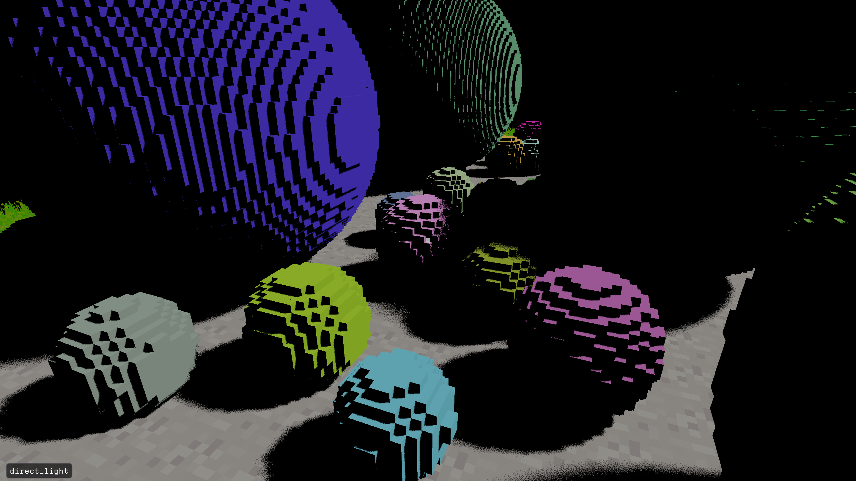
Above is what we get from the shadow tracer each frame. A binary mask telling us whether the ray hit the light source or not.

Indirect light

Direct lighting on its own is not that exciting. Neither is just adding a constant ambient term to the output like seen above. Global illumination is all the rage nowadays and it is one of these things you did not know you were missing until you actually see it in action. In short, global illumination is about simulating the indirect lighting in a scene, so light that has bounced around the scene before hitting the object.

Global illumination is tricky though and there are many ways of solving it (e.g. DDGI, LPV, Lumen). Inspired by the full potato GI in Tiny Glade I went out to make an even more potato solution. We cast rays randomly in a hemisphere to determine the incoming radiance and then we pray the denoiser can clean it up.

Denoising

Now we have two very noisy signals we need to denoise but we also have two properties we can exploit. The signal has both temporal and spatial coherence. The lighting is unlikely to change for a pixel over time and pixels on the same surface will likely have similar incoming light. Thus, a temporal filter allows us to accumulate samples over time if the camera does not move too much, and a spatial filter allows us to utilize samples from neighboring pixels if they belong to the same surface. The tricky part is the two IFs though. All the filters see is a 2D image so we need to be careful about what samples we actually can use.

Temporal filter

If the camera has not moved too much we can likely accumulate new samples on top of the samples of previous frames. The tricky part here is that the camera is expected to move so you will need to reproject the history of samples on top of your current frame (such as in TAA). This is simple enough if you have motion vectors for each pixel, but you are bound to get pixels where there is no valid history, such as edges of the frame or disoccluded areas.

In a perfect world the reprojection would only produce valid history; then it is just a matter of picking some strategy for accumulating the samples. I went for an exponential moving average. I record the number of samples collected and blend the history and the new samples according to lerp(old, new, 1 / num_samples). I also have a constant MAX_SAMPLES for clamping num_samples which allows me to control how fast we accumulate samples.

However, the world is not perfect and a big part of this filter is actually determining whether history is valid or not. Edges of the screen are straightforward, we just check if we try to sample outside the history texture. The tricky part is that it is a 3D scene, and as the camera (or objects) move, we get disocclusions (surfaces previously not seen). Thankfully we do deferred rendering so I have a lot of information about the scene at my disposal and can compare the depth and the normal in an attempt to detect disocclusions.

This is a typical trade-off. Collect a large set of samples and you get less noise but you will also react slower to changes in the scene. If this is slow enough you will get a lot of noticeable artifacts for areas where the history is reset rapidly.

Spatial filter

This filter is more like a blur filter. As mentioned, neighboring pixels likely hold the same incoming light (or lack thereof for shadows) and here we attempt to exploit this fact by aggregating together neighboring pixels. Here I went for two different approaches. The principle is the same but the two signals are a bit different so I will talk about this below.

Sadly we do not live in a perfect world and just as with the temporal filter it is not as simple as just blurring the image. You also need to consider how much to blur to not lose details and to make sure you do not blur across edges. The assumption is that a surface might have the same incoming light but the image contains many surfaces.

Shadow mask

Here I tried a bit of everything and in the end I ended up with something similar to SVGF. For the most part it is identical but I took some short cuts.

The temporal part is similar to what I have already described but with one addition. We also track the variance of the signal. The idea is that we can use the variance to guide the spatial filter.

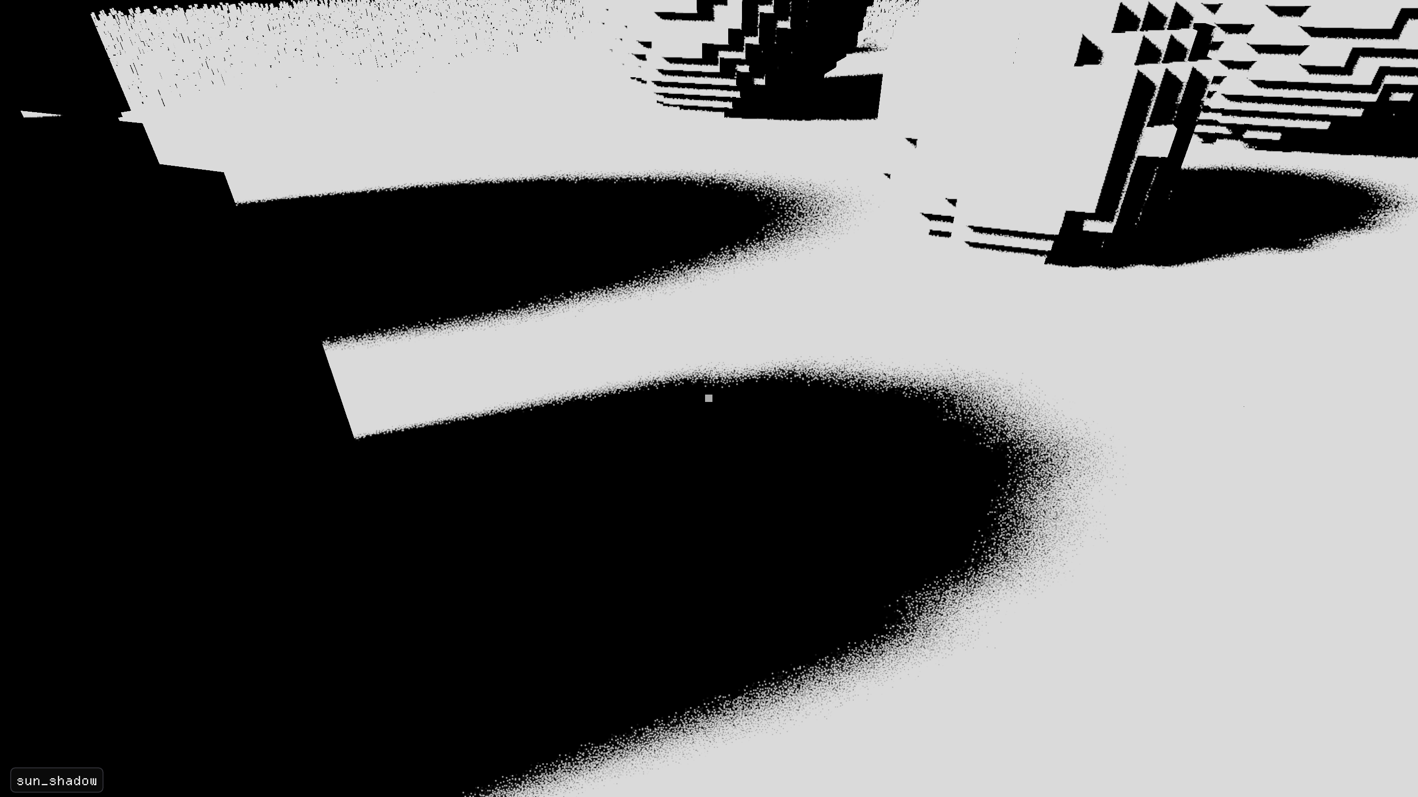
The spatial filter then uses a hierarchical À-Trous wavelet filter which uses our normals and depth to avoid filtering over edges. The variance we have collected is also used to control the degree of filtering. The idea is that areas with low variance, such as the shadow umbra, need less smoothing than areas with high variance (e.g. the penumbra). The first iteration of this filter is then what we keep as the history in the temporal filter for the next frame.

The tricky part here and with denoising in general is that there is a lot of tweaking involved. It all depends on your input signal and your scene and you have to tweak everything from your temporal accumulation to how to weight your spatial filter to get decent results.

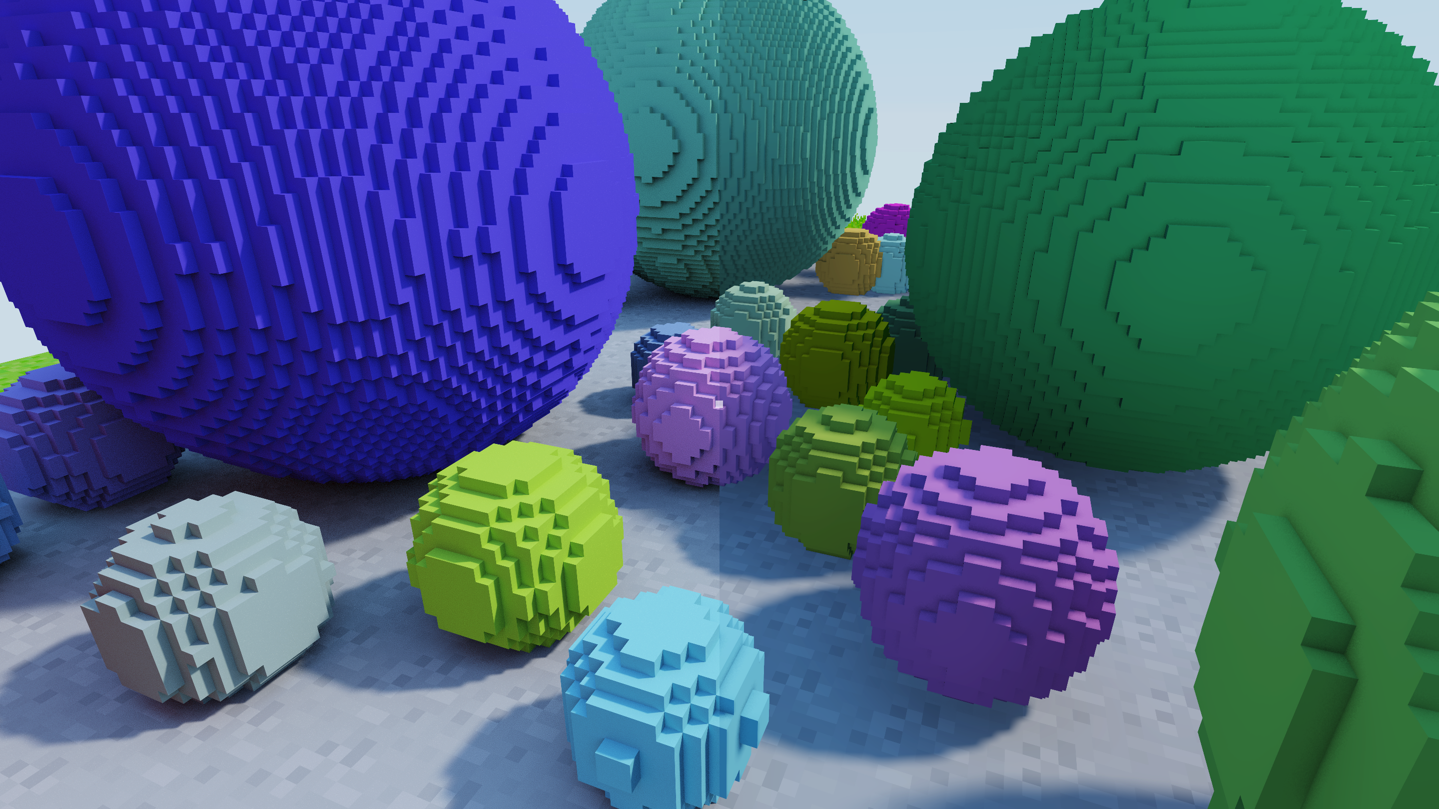
The penumbra looks a bit weird when looking at it like this so it might require some more tweaking. In the final render that is barely noticeable though.

Global illumination

The GI signal is a different beast. I tried the SVGF approach here as well and it looked straight-up terrible. One valuable thing to note about indirect lighting though is that it tends to be lower frequency. Visually I am way less worried about losing high frequency details and I am happy as long as I get a stable signal that is approximately correct.

One key aspect of denoising the GI is that I first project it into first-order spherical harmonics, which lets us preserve directional information, and this is what we feed into the denoiser. This is also what Tiny Glade and Metro Exodus did. The denoiser itself is also a bit more convoluted compared to SVGF. What I ended up with is similar to ReBLUR but with some simplifications.

The temporal filter is as described before but with some blur of the input before we accumulate it. This is due to the high number of outliers in the GI signal.

The spatial filter is a bit different though. We no longer use the variance to guide the spatial filter since the variance does not tell us much when it comes to GI compared to shadows where we have clear high and low variance areas. Instead we use the number of accumulated samples to control the size of the filter. The sampling for the filter is a bit different as well, we use a randomly rotated Poisson disk and we sample in world space as opposed to screen space. Similar to SVGF we also use the blurred image from the previous frame as the history in the temporal filter.

There are also some tricks to deal with disocclusions since the lack of samples is very noticeable in those areas. The ReBLUR paper suggests using a mip-chain but I went with just an ugly hack where I just collect neighboring samples. In principle it is the same, just more stupid.

Putting it together

Until now we have been rendering everything at half-resolution just because the raytracing is fairly expensive. So the first thing we need to do before actually putting everything together is to upsample our denoised targets. Here I use a simple bilateral filter. Using the normal and depth of the scene we can reliably upsample the image while keeping the edges.

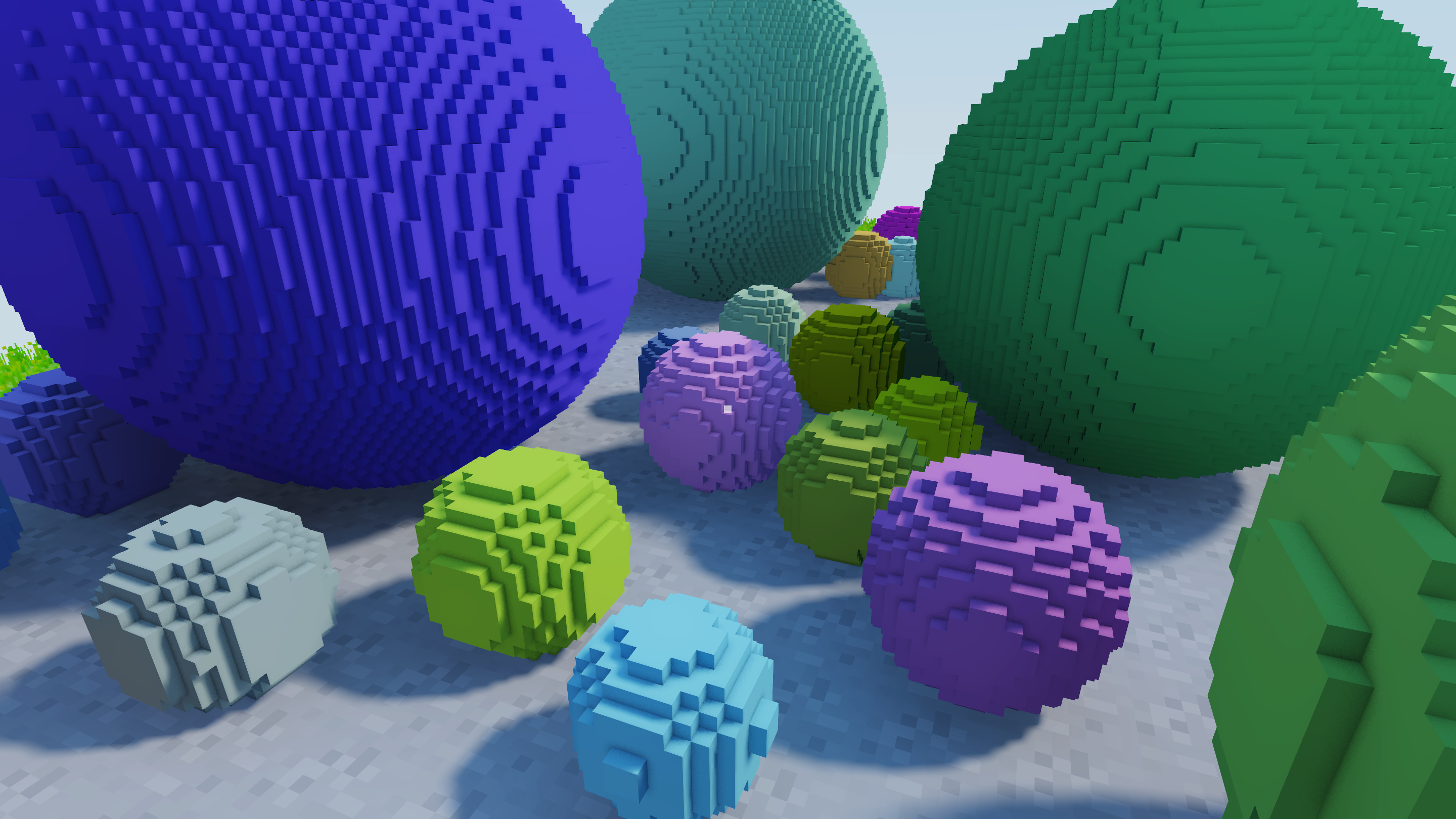
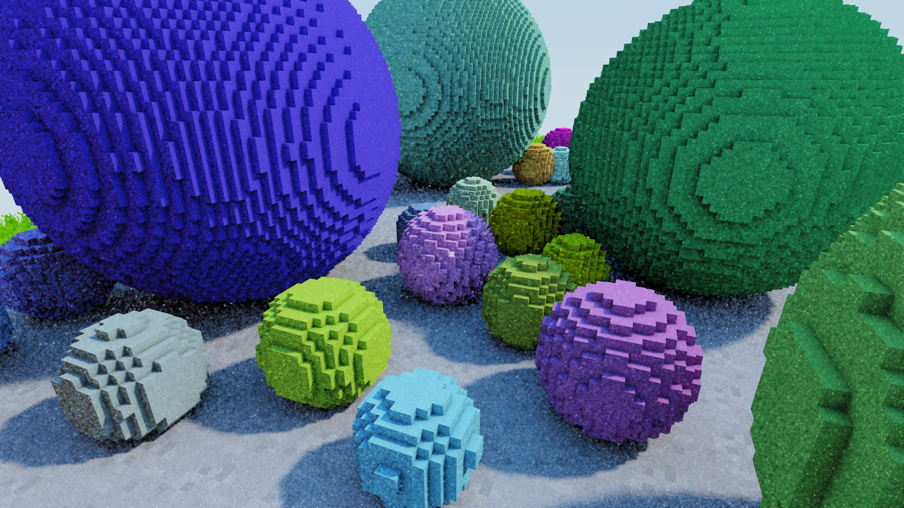
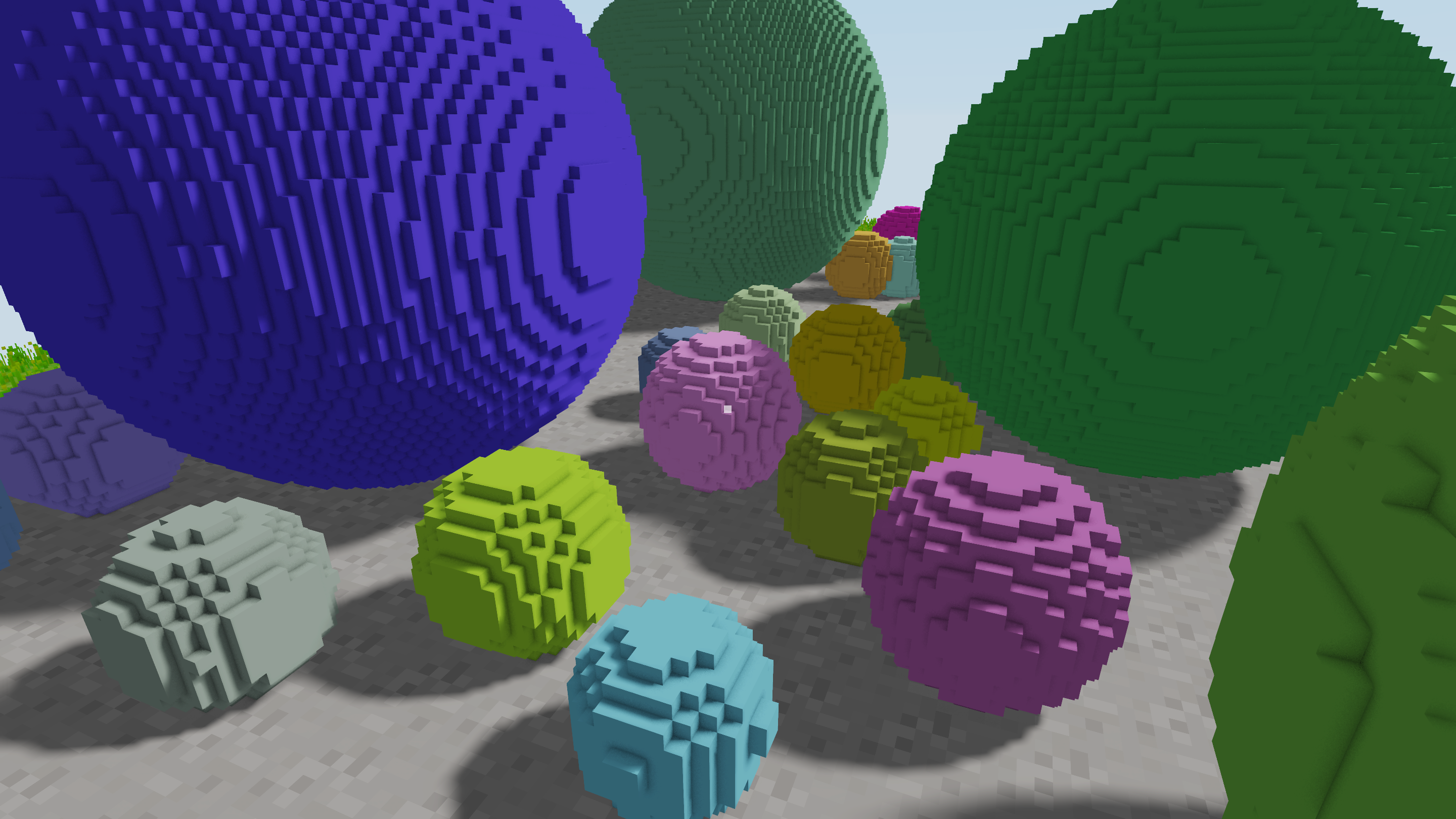
After all tracing, denoising, and upsampling we can finally composite the scene. We can compare our path traced reference (left) to the new render (right) and see that we are getting fairly close.

A visual difference is the ambient occlusion. One drawback of the heavy denoising is that we lose a lot of detail in the lighting so I am still relying on SSAO which lacks the visual depth of RTAO. I actually collect the hit distance during the GI trace so I could potentially attempt to denoise and reconstruct RTAO separately from the GI but that is something for the future.

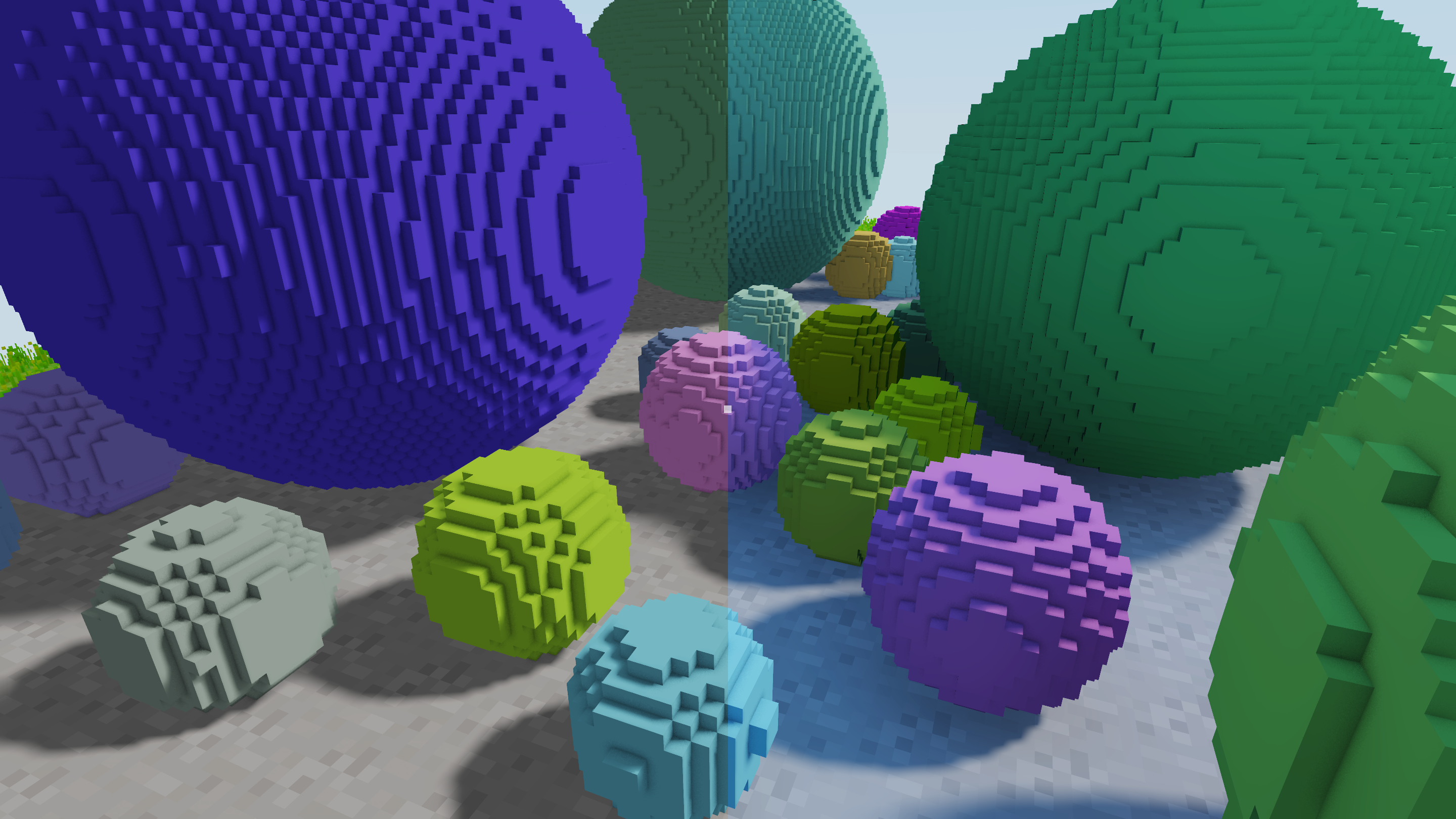
The old render (left) with the constant ambient term looks very dull in comparison to the new (right).

Coolest thing though, is that you can even see the bounce light in a Cornell box!

There is still better benchmarking needed but looking at some preliminary numbers, rendering the ball scene spends about 1.5 ms per frame on the GI trace and 0.5 ms on denoising at 2880x1620 (full res) on an RTX 3090. The sun shadow is about 0.5 ms in total (raycasting and denoising).

Limitations

It is worth nothing that even if we get some cool bounce lighting like in the Cornell box above, we still only do a single bounce so it will never look as good as a proper path tracer. This is not a deal breaker though as it can still look great. The issue is with noise and denoising artifacts. This whole thing was the result of a lot of experimentation and I expect that I will have to continue experimenting. The biggest issue now is dealing with indoor scenes.

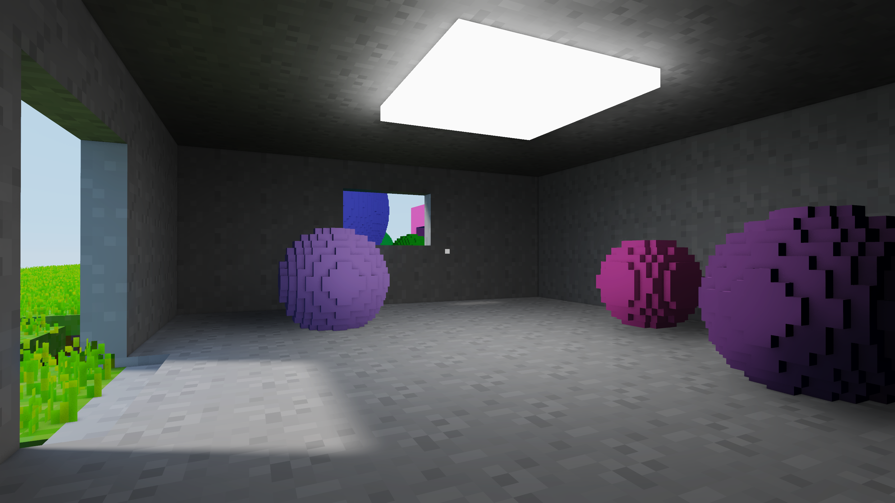
Indoor scenes are especially tricky due to the low amount of useful signal. While it is cool to see that I can now light a scene just using light-emitting voxels instead of analytical lights, you definitely see the lost details of the shadows caused by the denoiser.

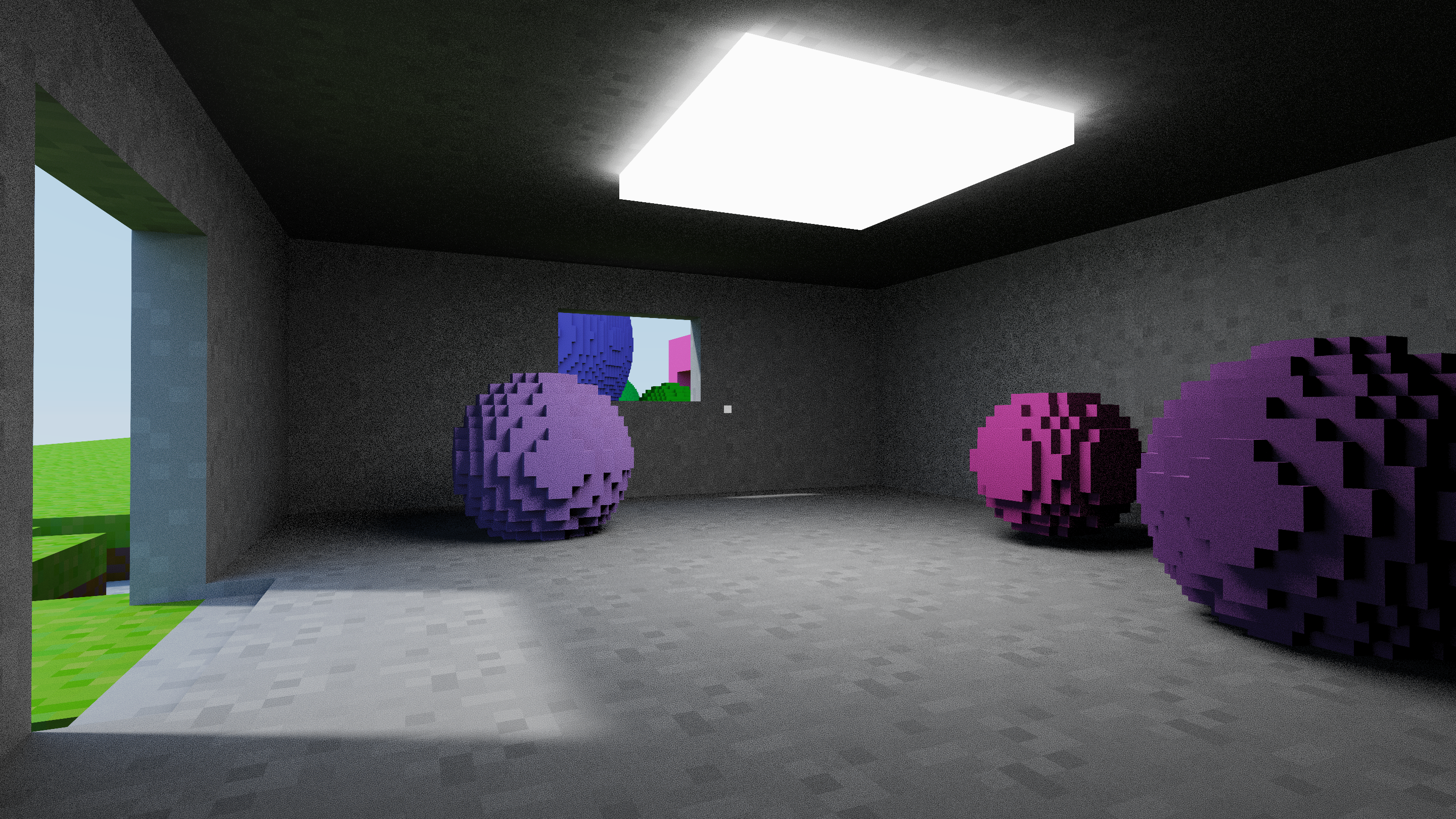
In the reference, the shadows, just like the previously mentioned AO, are a lot more defined.

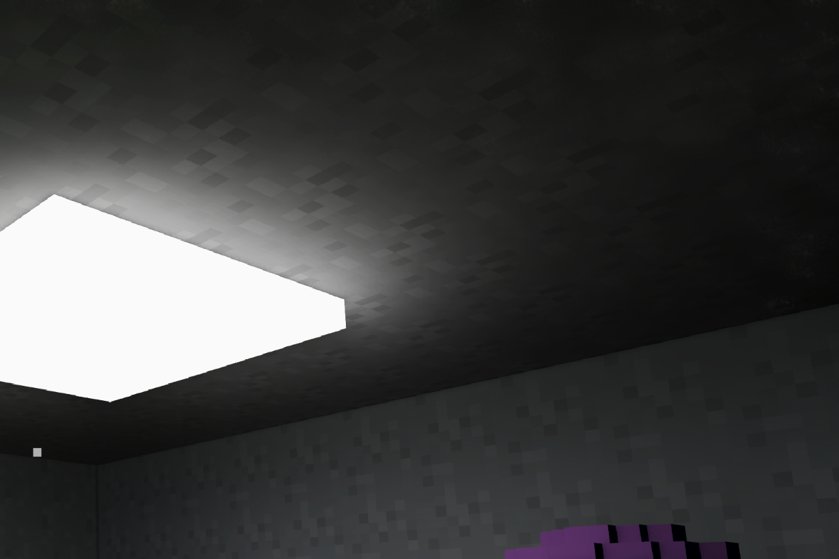
It is hard to spot in screenshots but there are also clear cases where the denoiser fails due to the low signal. Like in the image above you see some odd shifting patterns in the roof and this is even more noticeable when not looking at a still image. One issue here is that we rely on our random hemisphere rays actually hitting the light-emitting voxels. We might be able to reduce the noise by using importance sampling like they did for the Quake 2 raytracing demo.

AI

There are of course modern AI-based approaches for denoising out there such as NVIDIAs DLSS or AMDs Neural supersampling and denoising. However, I decided against them for now since you limit yourself to specific hardware. I might look into this more in the future.

Claude

In parallel to the work on the lighting I have continued experimenting with Claude Code with some mixed results.

Physics

I hinted briefly at Claude implementing a physics engine last month. Well, I made Claude implement it again, and again… After some micro-management and a detailed plan outlined by myself it actually managed to implement something that resembles actual game physics. There is a lot of weird dancing going on though.

It implements physics similar to how Teardown does it, with per-voxel collisions. Objects are just occupancy masks in 3D telling whether a voxel is solid or air. Then thanks to some ideas from Dennis Gustafsson it is actually feasible to calculate collisions per voxel (spoiler: you do not actually have to).

Have not had time to stress test this or anything but it is nice to now have the skeleton to actually be able to do so.

What’s next

I am happy with how it turned out for outdoor scenes but there is still some work to do indoors so I will fiddle around some more with the denoising. I have some ideas on what to try next. Other than that I might actually look a bit more into the physics. I recently read this captivating blog series by Glenn Fiedler so maybe I should add networking as well!

I also have this half-insane fully vibe coded project related to my previous synth project which I might continue directing. I will cover this in the next post if it actually goes somewhere.